HTS MODELING WORKGROUP: Shared Models
Shared Models
This page contains shared examples of numerical models. Feel free to download the files and use them. If you use them for your presentations/publications, please cite the related references.
Before submitting your files, please be advised:
Modelling examples must be associated with a peer-reviewed publication. Unpublished examples will be considered and approved by the Board;
All files will be checked before going online. Models made using unlicensed software will not be accepted under any circumstances.
Integral Equation for Thin Conductors Solved by Finite-Elements (Comsol)
2-D H-Formulation of Maxwell’s Equations with Edge Elements (Comsol, FlexPDE)
2-D Homogeneous Model to Estimate AC Losses in Coated Conductor Stacks and Coils (Comsol)
3-D Homogeneous Model to Estimate AC Losses in Coated Conductor Stacks and Coils (Comsol)
2-D Campbell’s Model to Estimate Magnetization Losses in a Wire in the Critical State (FreeFem++)
2-D Axisymmetric and 3-D Models for Magnetization of Superconducting Bulks (Comsol).
A Full 3-D Time-Dependent Electromagnetic Model for Roebel Cables (Comsol)
3-D H-Formulation for Superconducting Wires and the Gmsh Cohomology Solver (Gmsh)
2-D Electro-Thermal Model for Simulating Nonuniform Quench of 2G HTS CCs (Comsol)
A General Model for Transient Simulations of SFCL in Power Grids (Matlab/Gnu Octave)
A 2-D T-A Formulation Model for Modelling a 2G HTS Stack (Comsol)
T-A Multi-Scale and Homogeneous Models for the Benchmark #3 (Comsol)
MATLAB Scripts for Simulation of Superconductors (Tapes, Bars and Cylinders) (MATLAB 2016b or newer)
GetDP Scripts for Simulating Superconductors and Soft Ferromagnetic Materials (GetDP)
Open-Source 2D FDM Simulation for HTS Cables (MATLAB2016b or newer).
All the programs are distributed in the hope that they can be useful to the applied superconductivity community. They have been uploaded as received by the corresponding author and they are distributed without any warranty.
|—————————————————————————————————————–|
(1) – Integral Equation for thin Conductors Solved by Finite-Elements (shared by F. Grilli, Karlsruhe Institute of Technology).
The model calculates current density/field distribution in a superconducting thin conductors in the presence of a time-dependent transport current, background field or combination thereof (as in the figure below). The superconductor is modeled with a power-law. Dependence of Jc on magnetic field and position can be easily incorporated.
Model file (Comsol Multiphysics, version 4.3a): here.
Main reference: Brambilla et. al. 2008 Supercond. Sci. Tech. 21 (10) 105008.
The extension of the model to stacks/windings and radial/polygonal cables can be found in these two articles: Brambilla et al. 2009 Supercond. Sci. Tech. 22 (7) 075018; Brambilla et al. 2012 IEEE Trans. Appl. Supercond. 22 (4) 8401006. The approach is the same as in the case of a single tape, only the form of the kernel (expressing the electromagnetic interaction with the other tapes).
The figure shows the temporal evolution of the current density along the tape’s width under the simultaneous action of AC transport current and AC magnetic field.
|—————————————————————————————————————–|
(2) – 2-D H-Formulation of Maxwell’s Equations with Edge Elements (shared by F. Grilli, Karlsruhe Institute of Technology and P. Masson, Houston University).
The model calculates current density/field distribution in a superconducting wire in the presence of a time-dependent transport current, background field or combination thereof. The superconductor is modeled with a power-law. Dependence of Jc on magnetic field and position as well as the presence of other materials can be easily incorporated.
Model file (Comsol Multiphysics, version 4.3a): here.
Model file (FlexPDE, version 6): here.
Reference articles: Hong et al. 2006 Supercond. Sci. Tech. 19 (12) 1246-1252, Brambilla et al. 2007 Supercond. Sci. Tech. 20 (1) 16-24
The figure below the current density distribution as it changes during an AC cycle of the transport current.
|—————————————————————————————————————–|
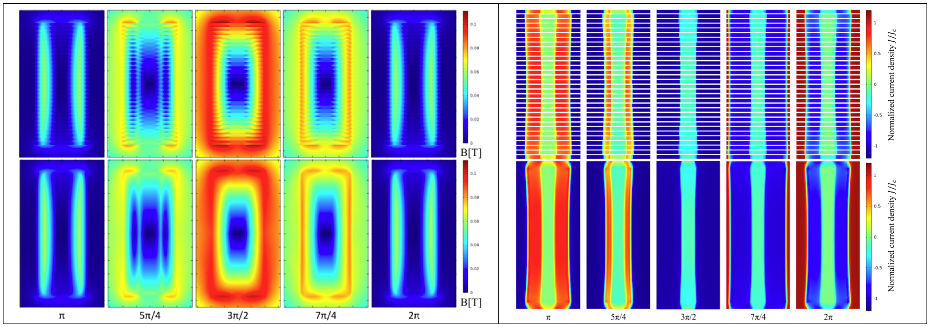
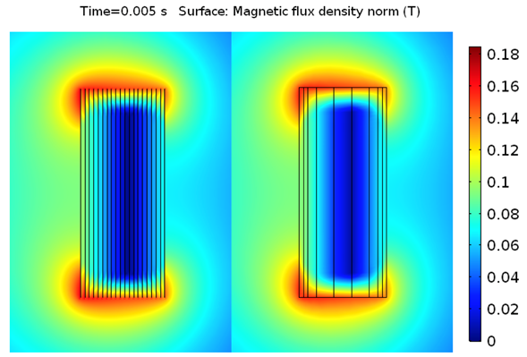
(3) – 2-D Homogeneous Model to Estimate AC Losses in Coated Conductor Stacks and Coils (shared by V. Zermeno, Karlsruhe Institute of Technology).
The model uses a homogenization technique to calculate the current distribution inside the superconducting layers of a HTS stack where each tape carries the same net current as it would be the case in a coil. The model estimates the AC losses of the stack. The homogenized model runs significantly faster than a reference model including the geometry of all the tapes in the stack.
Model file (Comsol Multiphysics, version 4.3a): reference and homogenized models.
Article about reference model: Rodriguez-Zermeno et al. 2011 IEEE Trans. Appl. Supercond. 21 (3) 3273-3276
Article about homogenized model: Zermeno et al. 2013 J. Appl. Phys. 114 173901
Exemplary result of the magnetic field and the normalized current density J/Jc(B) for a stack at different phase values
|—————————————————————————————————————–|
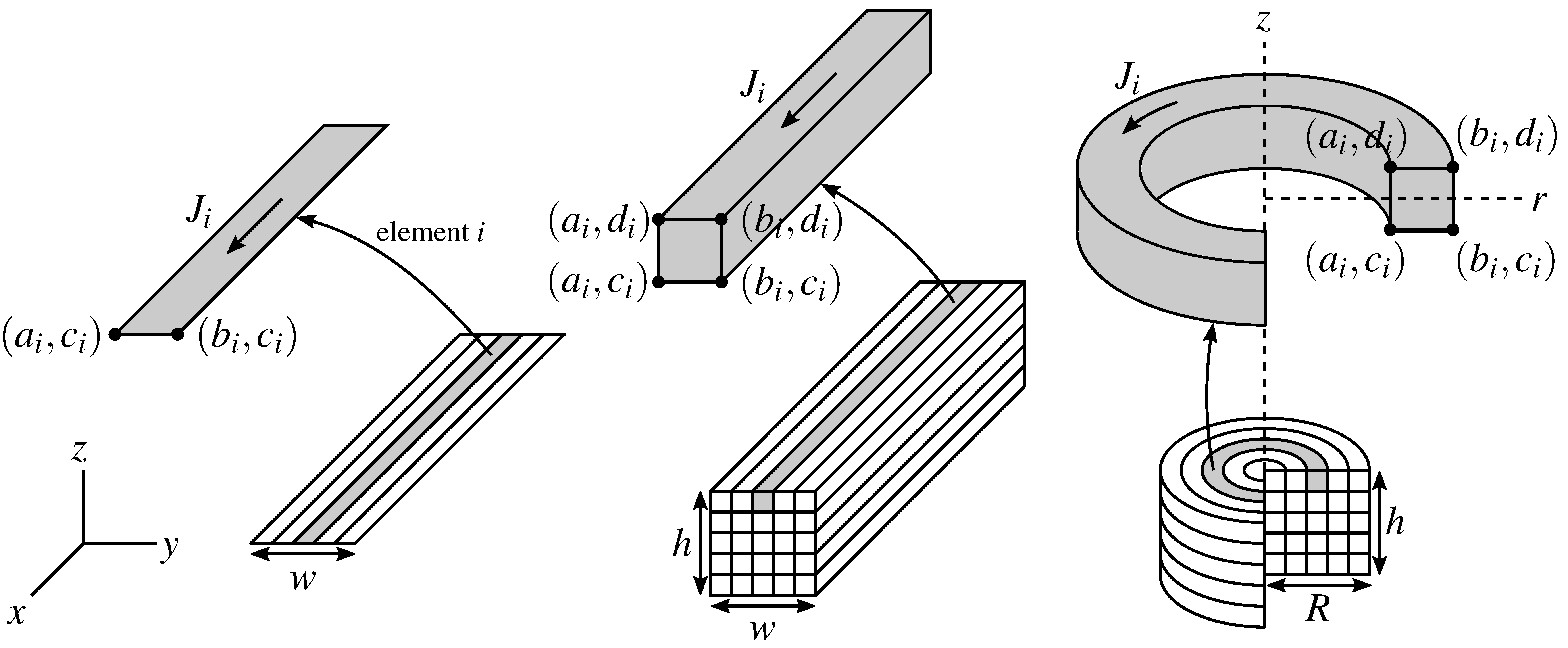
(4) – 3-D Homogeneous Model to Estimate AC Losses in Coated Conductor Stacks and Coils (shared by V. Zermeno, KIT).
This model uses a homogenization technique to calculate the current distribution inside the superconducting layers of a racetrack coil and to estimate its AC losses.
Model file (Comsol Multiphysics, version 4.3a): here.
Reference article: Zermeno and Grilli, 2014 Supercond. Sci. Technol. 27 044025
The figure shows the normalized current density J/Jc(B) for a quarter of the coil geometry. The sign is used to indicate the direction of the current.
|—————————————————————————————————————–|
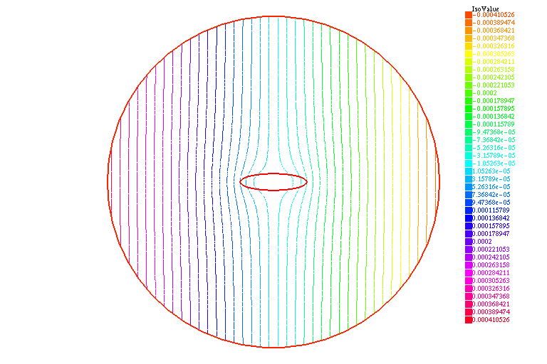
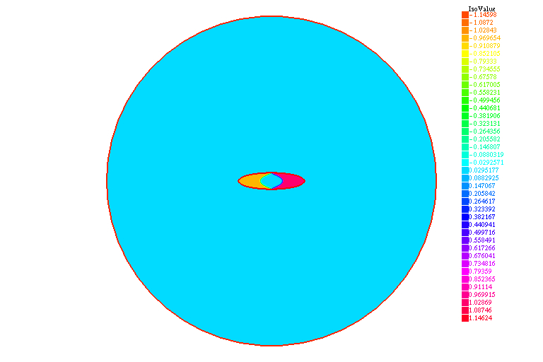
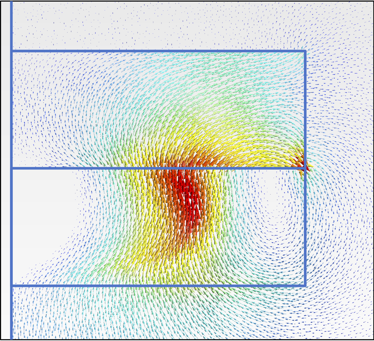
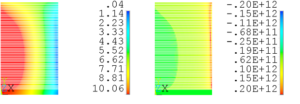
[**5] – 2-D Campbell’s Model to Estimate Magnetization Losses in a Wire in the Critical State (shared by E. Rizzo).**
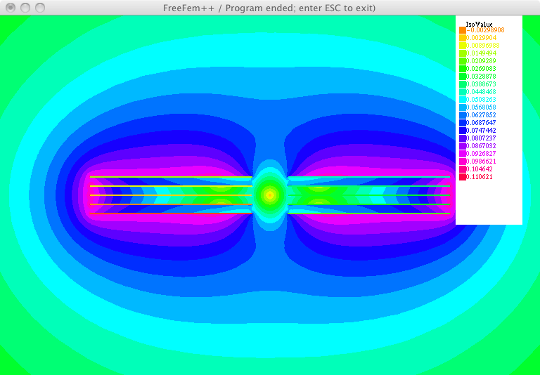
The model calculates the penetration of the magnetic field in the cross-section of a superconducting wire in the critical state subjected to a transverse magnetic field.
Model file (FreeFem++, version 3.38-1): here.
Reference articles: A. M. Campbell, 2007 Supercond. Sci. Technol. 20 292-295 and Francesco Grilli and Enrico Rizzo 2020 Eur. J. Phys. 41 045203
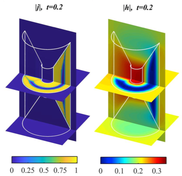
The figures below show the magnetic vector potential (left) and the current density distribution (right) in an elliptical superconductor subjected to a vertical uniform magnetic field.
|—————————————————————————————————————–|
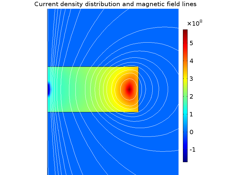
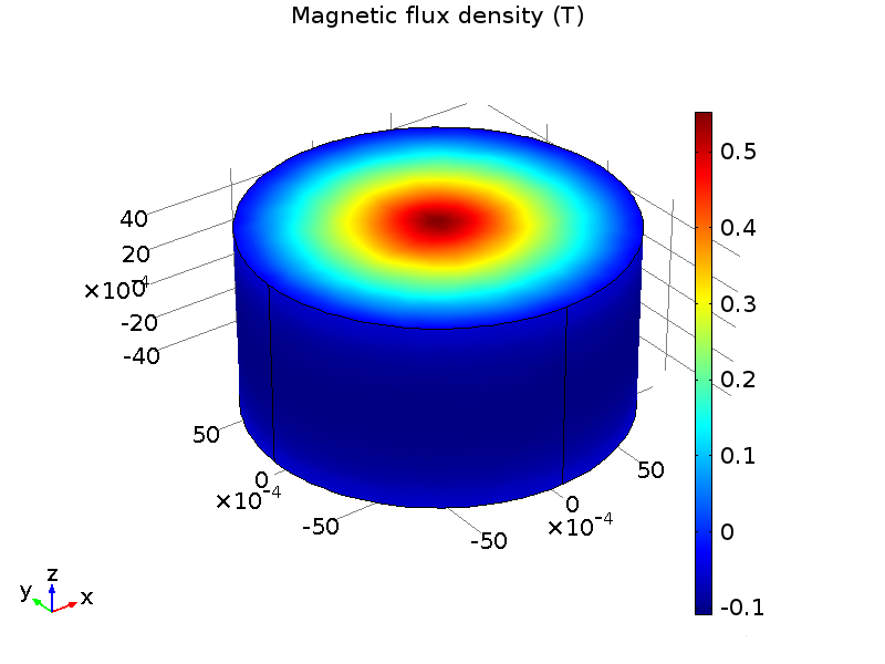
[6] – 2-D Axisymmetric and 3-D Models for Magnetization of Superconducting Bulks (shared by M. Ainslie, University of Cambridge).
The first model is for a 2D axisymmetric bulk with zero field cooling (ZFC) magnetization. Here, the external magnetizing field is applied along the z axis – perpendicular to the top/bottom surface of the bulk – assuming the bulk is already cooled to its particular operating temperature. Based on the Bean model, the external magnetizing field required is at least twice the trapped field capability of the bulk for full magnetization. The applied field is simply a triangular waveform. The second model is for a 3D bulk with pulsed field magnetization (PFM). Here, the external field is also applied along the z axis, but the time scale is much shorter. Both models do not include the thermal model
Model file 2-D (Comsol, version 4.3a): here.
Model file 3-D (Comsol, version 4.3a): here.
Reference articles for the 2-D model: Philippe et al. 2015 Supercond. Sci. Technol. 28 (9) 095008, Zou et al. 2015 Supercond. Sci. Technol. 28 (7) 075009.
Reference article for the 3-D model: Ainslie et al. 2014 Supercond. Sci. Technol. 27 (6) 065008.
|—————————————————————————————————————–|
[7] – A Self-Consistent Model to Estimate the Critical Current of Superconducting Devices (shared by V. Zermeno, Karlsruhe Institute of Technology).
The model presented here is used to estimate the critical current of superconducting devices. Its implementation is very simple either using finite-element-based or general numerical analysis programs. The model runs very fast, even on a laptop computer, making it a useful tool for optimization. In general, the model is very flexible and can be applied to many superconducting devices including transposed cables, single tape coils, coils made of transposed cables, non-transposed cables and cables with ohmic termination resistances. The main description of the model can be found here http://iopscience.iop.org/article/10.1088/0953-2048/28/8/085004
Several implementations for estimating the critical current of a 10 strand Roebel cable using COMSOL, MATLAB/Octave and FreeFEM++ are given below. The codes are fully commented and described here: http://arxiv.org/ftp/arxiv/papers/1509/1509.01856.pdfModel file 2-D (FreeFem++, Matlab/Gnu Octave, Comsol version 4.3a): here.
|—————————————————————————————————————–|
[8] – A full 3D Time-Dependent Electromagnetic Model for Roebel Cables (shared by V. Zermeno, Karlsruhe Institute of Technology).
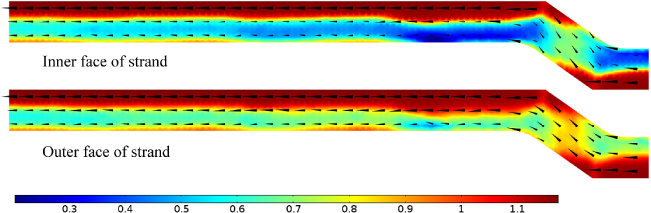
This model simulates the current distribution in the superconducting layers of a Roebel cable composed of 14 strands and estimates its AC losses. The mode is rather general and allows considering the cases of current transport or externally applied field. The figure shows the normalized current density J/Jc(B) at peak value of an applied net transport current with amplitude of 400 A (86% of Ic). Note the profile difference between both faces of the same strand. The color scale shows the magnitude of the current density. Cones indicate the direction of the current density vector.
Model file (Comsol Multiphysics, version 4.3a): here.
Reference article: Zermeno et al. 2013 Supercond. Sci. Technol. 26 052001.
|—————————————————————————————————————–|
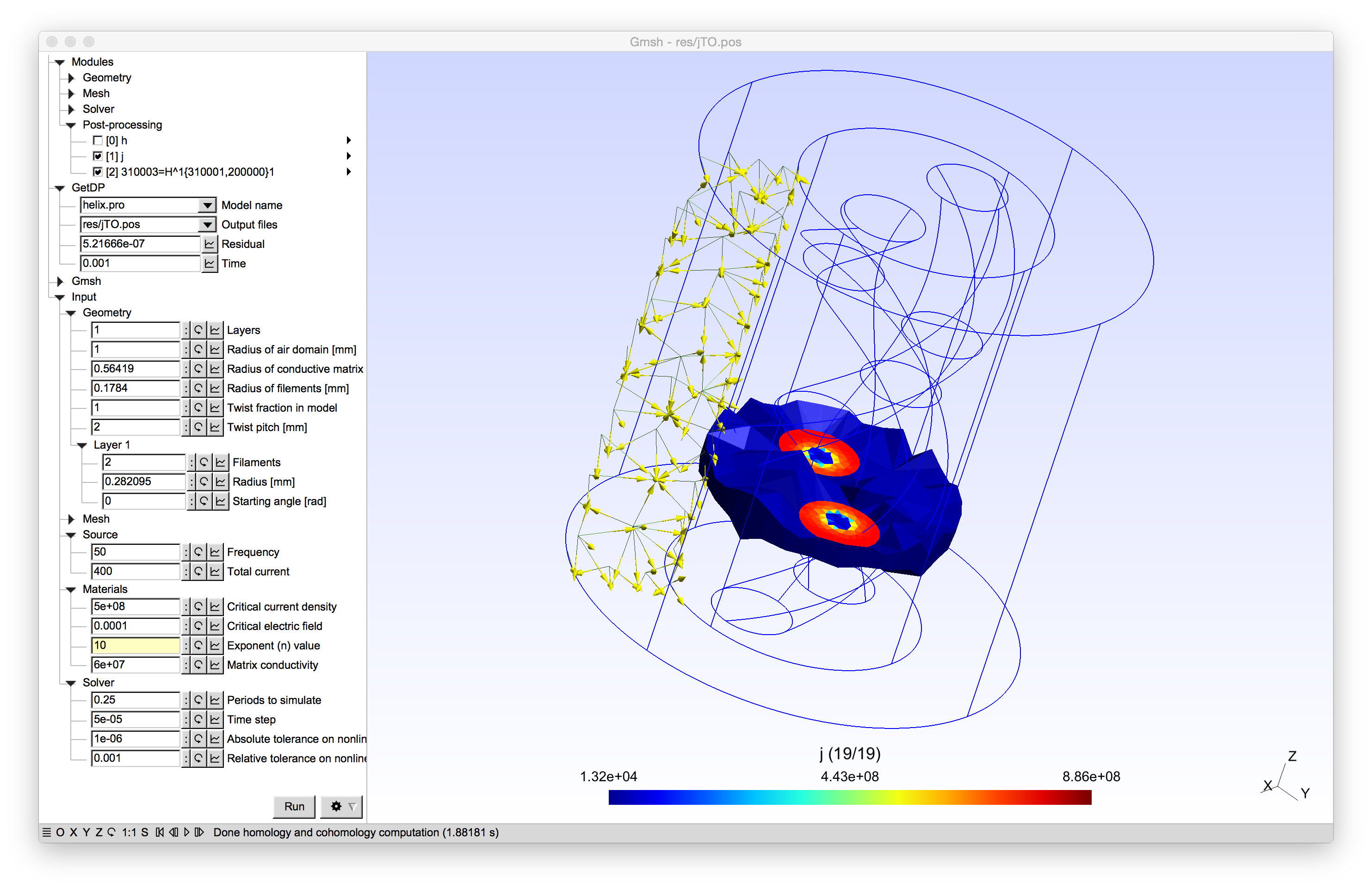
[9] – 3D H-Formulation for Superconducting Wires and the Gmsh Cohomology solver (shared by C. Geuzaine, University of Liège) The nonlinear power-law resistivity in the superconducting filaments is linearized as in this paper.
Model file and instructions: here.
Presentation given by C. Geuzaine at EUCAS 2015, Lyon, France: here.
|—————————————————————————————————————–|
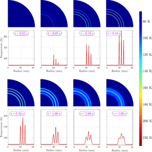
[10] – 2-D Electro-Thermal Model for Simulating Nonuniform Quench of 2G HTS CCs (shared by C. Lacroix, Polytechnique Montréal, F. Sirois, Polytechnique Montréal and F. Grilli, Karlsruhe Institute of Technology).
The model calculates the time evolution of the electric potential and the temperature in a 2G HTS CC when a transport current is applied in presence of a low Jc region (defect) in the tape. The heat generated at the defect location creates a normal zone that propagates along the tape. The model can be used to determine the normal zone propagation velocity (NZPV) and the minimum quench energy for given geometric parameters of the tape. One important feature of the model is the possibility to adjust the interface resistance between the HTS layer and the stabilizer layer, which has an important impact on NZPV.
Model file (Comsol Multiphysics, version 4.3b with Joule Heating module) : here
Reference article: Lacroix et al. 2014 Supercond. Sci. Tech. 27 (3) 035003
The figure below shows the temperature distribution of the HTS tape over time when a transport current close to the critical current is injected into the tape. The low Jc region induced a normal zone on the right end of the tape, which then propagates along its length.
|—————————————————————————————————————–|
[11] – A Parameter-free Method to Extract the Superconductor’s Jc(B,θ) Field-dependence from in-Field Current–Voltage Characteristics of High Temperature Superconductor Tapes (shared by V. Zermeno, Karlsruhe Institute of Technology and K. Habelok, Silesian University of Technology).
The method presented here allows computing the critical current density (Jc) of superconducting materials from its in-field experimentally measured critical current (Ic). This is particularly important for applications like HTS cables for power transmission and fault current limiters, where superconductors experience a local field that is close to the self-field of an isolated conductor. Therefore it is necessary to solve an inverse problem to correct for the contribution derived from the self–field. Here, a method that involves minimum regularization and no human interaction or preconception of the Jc dependence with respect to the magnetic field is presented. This parameter-free approach provides excellent reproduction of experimental data and runs in a few minutes.
The script file (Matlab, version 2015a and Comsol Multiphysics, version 5.2a with Livelink for Matlab) and some sample data values are given: here
Reference article: Zermeno et al. 2017 Supercond. Sci. Tech. 30 034001
|—————————————————————————————————————–|
[12] – This Model Simulates the Behaviour of a Superconducting Fault Current Limiters (SFCL) Connected to a Power System (shared by W. T. B. de Sousa, Karlsruhe Institute of Technology).
The model can be implemented in any power system simulator (e.g., Matlab/Simulink, EMTP, PowerFactoy, etc.) for transient analyses of short circuit currents. Here one presents the method applied to MCP-BSCCO-2212 SFCL devices. The method however has already been extended to SFCL based on 2G tapes (see for example 10.1109/TASC.2014.2311396 and 10.1109/TASC.2014.2387311).
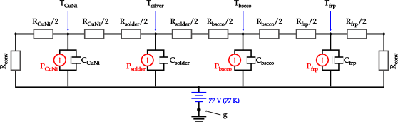
A non-adiabatic model is used in order to simulate the thermal behavior of the SFCL device properly. The model takes into account the characteristic E–J curve of the HTS material as well as the strong coupling between electrical and thermal phenomena. The one dimensional time-dependent heat transfer across the layers of the tapes is modeled by the so called Thermal-electrical Analogy. The equivalent RC circuits shown in the figure represent the thermal analogy for the MCP-BSCCO-2212 SFCL. Resistances correspond to heat conduction of each material, while capacitors correspond to respective thermal capacity. The convective heat transfer between the modules and LN2 is modeled as convective resistances. Internal heat generation at each layer is represented by current sources. The dc voltage sources simulate the LN2 bath (77 K). The temperature rise of each layer is calculated as a voltage drop between Tlayer and g.
Model file (Matlab/GNU Octave) script: here
Reference article: de Sousa et al. Cryogenics 62 97-109
|—————————————————————————————————————–|
[13] – The Model Calculates Current Density, Field Distribution, and Levitation Force in a Superconducting Magnetic Bearing (SMB) Composed by a Permanent Magnet an HTS Sample (shared by Guilherme Goncalves Sotelo, Universidade Federal Fluminense, Niterói, Rio de Janeiro, Brazil).
In the considered examples, the HTS sample is either a bulk superconductor or stacks of 2G wires. In the second case, the 2G stack was homogenized in order to speed up the solution. The movement between the HTS and the permanent magnet is avoided in the model by restricting the simulation domain to the HTS itself, which can be done by applying appropriate boundary conditions.
Available here are two Matlab scripts that can be used two build up the 10 COMSOL models presented in the reference paper. The first file (“SMB_BULK_test_1_to_5.m”) allows the simulation of tests 1 to 5, using the bulk superconductor. The second file (“SMB_2G_STACKS_test_6_to_10.m”) models the SMB built with 2G stacks and can be used to simulate tests 6 to 10.
Model files (COMSOL 4.4 with MATLAB): here.
Reference article: Sass et al. 2015 Supercond. Sci. Technol. 28 125012
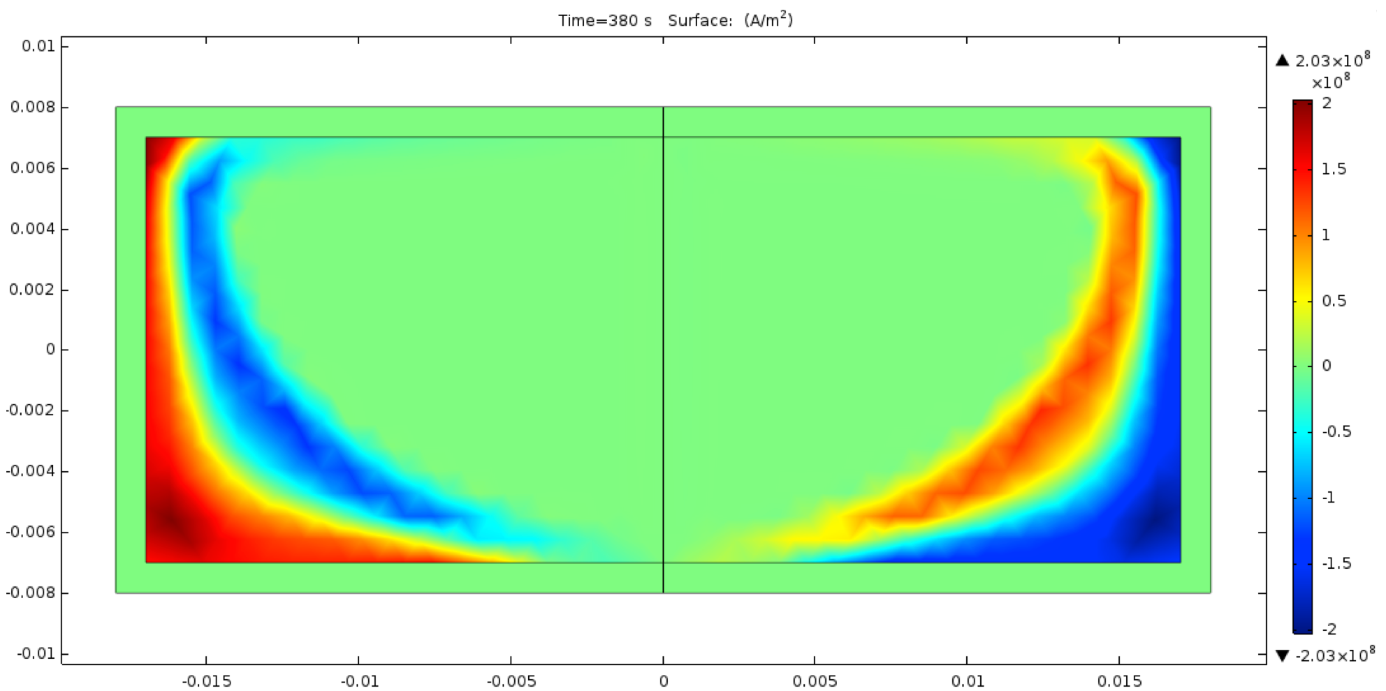
The figure below shows an examples of induced current density profiles for the SMB built with bulk.
|—————————————————————————————————————–|
[14] – Modeling and Simulation of Termination Resistances in Superconducting Cables (shared by V. Zermeno and Philip Krüger, Karlsruhe Institute of Technology, and by M. Takayasu, Massachusetts Institute of Technology).
The models presented here are used to simulate termination resistances which are largely responsible for the uneven distribution of currents in superconducting cables [1]. For this purpose, four different models are presented. The first is a 0D stationary model, where time enters as a parameter driving the net current in the cable. Being the simplest and fastest, it can be used to obtain a qualitative estimate of the current distributions (described in [2]). The second model, also stationary, is a 2D approach that considers both the actual cross section of the cable, and the dependence of the critical current density with respect to the magnetic field (described in [3]). The third model, also in 2D, is a quasi-static approach where an additional term is added to the electric field to take into account the voltage drop due to termination resistances (described in [2]). The fourth model, also quasi-static, is a 3D approach. Using two non-connected domains, it simulates both the termination resistances and the superconducting cable to calculate the current share in the cable’s strands (described in [2]).
Several implementations for estimating the current share in a 4 tape TSTC cable using Mathematica (0D) and COMSOL (2D and 3D), along with the corresponding experimental data [1] are given here.
Reference articles:
[1] Takayasu et al. 2012 Supercond. Sci. Technol. 25 014011
[2] Zermeno et al. 2014 Supercond. Sci. Technol. 27 124013
[3] Zermeno et al. 2015 Supercond. Sci. Technol. 28 085004
|—————————————————————————————————————–|
[15] – Using the Recently Proposed Fast Fourier Transform Based Three-dimensional Numerical Method [Prigozhin and Sokolovsky, ArXiv 1801.04869] the performance of a magnetic shield and a magnetic lens made of a bulk type-II superconductor is modeled (shared by L. Prigozhin, Ben-Gurion University of the Negev).
The method is efficient and can be easier to implement than the alternative approaches based on the finite element methods.
Matlab files: here.
Reference article: L. Prigozhin and V. Sokolovsky, ArXiV 1803.01346
|—————————————————————————————————————–|
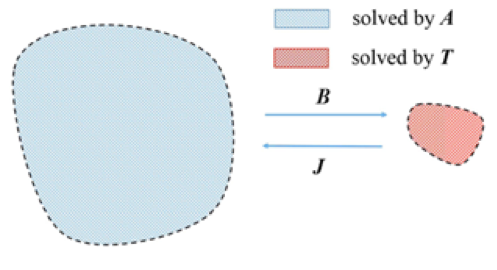
[16] – A Mixed A- and H-Formulation Approach for Modeling Electrical Machines with Superconducting Windings (shared by R. Brambilla, Ricerca sul Sistema Energetico, Italy).
The model uses the H-formulation for the superconducting windings and the A-formulation for the non-superconducting parts. Two important lines are defined: the “tramodel” lines, which separates the two formulations, and the “rotation” line, which separates the fixed and rotating parts.
Comsol files (version 5.3): here.
Reference article: Brambilla et al., 2018 IEEE Trans. Appl. Supercond. 28 (5) 5207511
|—————————————————————————————————————–|
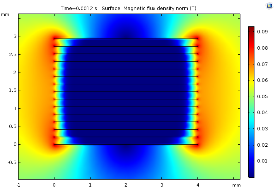
[17] – A T-A Formulation Model for Modelling a 2G HTS Stack (shared by Min Zhang, University of Strathclyde, UK).
The model shows how to use the thin strip approximation for the superconducting coated conductors to speed up calculation. The model simulates the magnetisation of a 2G HTS stack. The T formulation is used for modelling superconducting domains and the A formulation is used for modelling other domains. The model is implemented in Comsol 5.3a: the T formulation is solved by the PDE module and the A formulation is solved by the AC/DC module.
Comsol files (version 5.3a): here.
Reference article: Liang et al. 2017 J. Appl. Phys. 122 043903
|—————————————————————————————————————–|
[18] – Effect of tape non uniformities on end-to-end V-I characteristics of superconducting tape (shared by Francesco Grilli, Karlsruhe Institute of Technology).
This code evaluates the influence of non-uniformities of (Ic,n) along a superconducting tape, modeled as a series of non-linear resistances, each characterized by its Ic and n. In particular, it calculates the effect of the statistical distributions of Ic and n of these segments on the end-to-end Ic and n of the tape. The code is developed for normal and Weibull distributions, but it can be easily adapted to be used with other types of statistical distributions and with measured data.
MATLAB/Octave file : here.
|—————————————————————————————————————–|
[19] – AC Losses in a Superconducting Magnet in the Presence of a Time-Dependent Transport Current (shared by Lingfeng Lai, Beijing Eastforce Superconducting Technology Co., Ltd.(EFST)).
This model is based on ANSYS 15.0. The model calculates the AC loss in a superconducting magnet in the presence of a time-dependent transport current. The superconductor is modeled with Bean model. The parameters and outputs are all in text format, can be easily read and modified. Almost no knowledge beforehand is required. With some experience of using ANSYS ADPL, it can be easily modified to calculate the macro electromagnetic properties of superconductor, superconducting magnet flux penetration, AC loss and critical current. It is helpful for the further study of superconducting power equipment dynamics, AC applications and magnet shielding current effect.
ANSYS 15.0 File : here.
|—————————————————————————————————————–|
[20] – T-A Multi-Scale and Homogeneous Models for the Benchmark #3 (shared by Edgar Berrospe, National Autonomous University of Mexico, Mexico).
These two models address the analysis of the Benchmark #3, a 20 HTS tapes stack. The models show how the multi-scale and homogeneous methods are adapted to be used in conjunction with the T-A formulation. The achieved simplification in the description of the system allow to reduce the computation time.
Comsol files (version 5.2a): here.
Reference article: Edgar Berrospe-Juarez et al 2019 Supercond. Sci. Technol. 32 065003
|—————————————————————————————————————–|
[21] – MATLAB Scripts for Simulation of Superconductors (Tapes, Bars and Cylinders) (shared by Simon Otten, University of Twente, Netherlands).
Scripts for Matlab to simulate superconducting strips, bars and cylinders in various conditions of applied magnetic fields and currents. To find the current distribution, an integral formulation known as Brandt’s method is used.
Matlab Files (version 2016b or newer): here.
|—————————————————————————————————————–|
[22] – GetDP Scripts for Simulating Superconductors and Soft Ferromagnetic Materials (shared by J. Dular, University of Liège, Belgium).
Models based on GetDP as a finite element solver and Gmsh as a mesh generator. The models include an E-J power law for superconductors and an anhysteretic law for ferromagnetic materials. The finite element method is implemented either with an A- or an H-formulation, for tapes, cylinders, and cubes. One model includes a coupled A-H formulation.
Files available here.
|—————————————————————————————————————–|
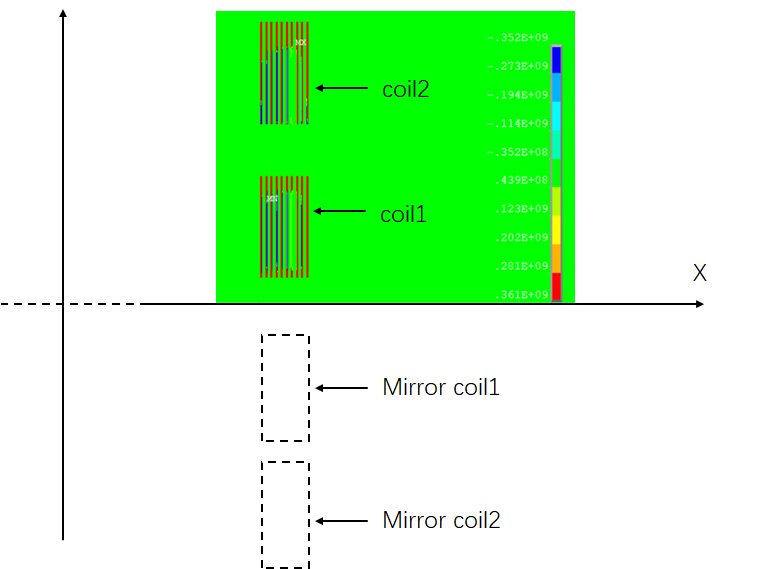
[23] – ANSYS APDL Codes for Modelling the Critical State Magnetization Current in REBCO Tape Stacks with a Large Number of Layers Using the A-V Formulation (shared by Kai Zhang, Paul Scherrer Institut, Switzerland).
An iterative algorithm method, based on ANSYS A–V formulation, is developed to simulate the critical state magnetization current J_c(_B,θ) in ReBCO tape stacks during the field-cooling magnetization. The computation speed is quite fast because the eddy current is not computed in non-superconductor region and no resistivity-nonlinear (E-J power law) exists in the FEA model. The iterative algorithm utilizes the function of multi-frame restart analysis in ANSYS.
ANSYS APDL files (version 18.1 Academic): here
Reference article: Zhang K et al. 2020 Magnetization simulation of ReBCO tape stack with a large number of layers using the ANYS A-V-A formulation IEEE Trans. Appl. Supercond. 30 4700805
|—————————————————————————————————————–|
[24] – Open-Source 2D FDM Simulation for HTS Cables (shared by W. T. B. de Sousa, Karlsruhe Institute of Technology).
In this work a two-dimensional open source simulation code based on the finite difference method (FDM) has been developed. It is solved by means of the alternating direction implicit routine (ADI). The algorithm has been written in MATLAB language. The method improves computational performance and simulation time. In addition, this enables the creation of open-source simulation codes. A three-phase concentric HTS cable design has been chosen for the development of the code, nevertheless the model can be employed for any cable design. The results indicate an efficient, stable and powerful simulation code. During the development no numerical instabilities have been found. Besides that, the model is able to deliver quantities that are experimentally difficult to access.
Matlab Files (version 2016b or newer): here