Smith Chart – plots with Matlab
2.- Calculate Reflection Coefficient, VSWR and Return loss
3.- Video: alternative code to draw the chart
1.- Useful for visualization of radio frequency and transmission line problems
The Smith chart was created by Phillip H. Smith in 1939. It’s a graphical tool designed for electrical engineers specializing in radio frequency (RF) to solve problems related to transmission lines and matching circuits.
Use of the Smith chart has grown over the years and it’s still used today, not only as a problem solving tool, but as a graphical display to show how RF parameters behave at one or more frequencies.(adsbygoogle=window.adsbygoogle||[]).push({});
The Smith chart can be used to represent many parameters including impedances, admittances, reflection and transmission coefficients, scattering parameters…Normalized scaling allows the Smith chart to be used for problems involving any characteristic or system impedance which is represented by the center point of the chart. The most commonly used normalization impedance is 50 ohms. Once an answer is obtained through the graphical method, it is easy to convert between the normalized impedance and the corresponding unnormalized value by multiplying by the characteristic impedance. Reflection coefficients can be read directly from the chart.
Use of the Smith chart and the meaning of the results obtained requires a good understanding of AC circuits and transmission line theory, both of which are needed by RF engineers.
In the chart, there are horizontal circles that represent constant resistances; vertical circles represent constant reactances. The complex impedance (or admittance )is normalized using a reference, which usually is the characteristic impedance Z0.
The chart is part of current CAD tools and modern measurement equipments. It’s a graphic of the reflection coefficient in polar coordinates.
Let’s create a chart with Matlab.
function draw\_smith\_chart

% Draw outer circle
t = linspace(0, 2\*pi, 100);
x = cos(t);
y = sin(t);
plot(x, y, 'linewidth', 3); axis equal;

% Place title and remove ticks from axes
title(' Smith Chart ')
set(gca,'xticklabel',{\[\]});
set(gca,'yticklabel',{\[\]});
hold on

% Draw circles along horizontal axis
k = \[.25 .5 .75\];
for i = 1 : length(k)
 x(i,:) = k(i) + (1 - k(i)) \* cos(t);
 y(i,:) = (1 - k(i)) \* sin(t);
 plot(x(i,:), y(i,:), 'k')
end

% Draw partial circles along vertical axis
kt = \[2.5 pi 3.79 4.22\];
k = \[.5 1 2 4\];
for i = 1 : length(kt)
 t = linspace(kt(i), 1.5\*pi, 50);
 a(i,:) = 1 + k(i) \* cos(t);
 b(i,:) = k(i) + k(i) \* sin(t);
 plot(a(i,:), b(i,:),'k:', a(i,:), -b(i,:),'k:' )
end
2.- Calculate the Reflection Coefficient, VSWR and Return Loss
Now, let’s prepare some formulas to calculate typical values used in RF theory. To plot a reflection coefficient we need a normalized impedance with magnitude and angle. It’s a good idea to deliver the angle in degrees to make it easier to visualize, and also let’s calculate the Voltage Standing Wave Ratio (VSWR) and the return loss.
function \[m, thd, SWR, rloss\] = smith\_ch\_calc(Z0, Zl)

% Draw appropriate chart
draw\_smith\_chart

% Normalize given impedance
zl = Zl/Z0;

% Calculate reflection, magnitude and angle
g = (zl - 1)/(zl + 1);
m = abs(g);
th = angle(g);

% Plot appropriate point
polar(th, m, 'r\*')

% Change radians to degrees
thd = th \* 180/pi;

% Calculate VSWR and return loss.
% We can add epsilon to magnitude, to avoid div by 0 or log(0)
SWR = (1 + m)/(1 - m + eps);
rloss = -20 \* log10(m + eps);
Now, let’s try our functions:
clear, clc, close all, format compact
\[m1, d1, VSWR1, Rloss1\] = smith\_ch\_calc(50, 50)
\[m2, d2, VSWR2, Rloss2\] = smith\_ch\_calc(50, 100 + 50j)
\[m3, d3, VSWR3, Rloss3\] = smith\_ch\_calc(50, 30 - j\*47)
and the results are:
m1 = 0
d1 = 0
VSWR1 = 1.0000
Rloss1 = 313.0712

m2 = 0.4472
d2 = 26.5651
VSWR2 = 2.6180
Rloss2 = 6.9897

m3 =     0.5505
d3 =   -82.6171
VSWR3 =  3.4494
Rloss3 = 5.1848
3.- Video: alternative code to draw the chart
This video shows an alternative code to draw the Smith Chart. You can pause the video to take appropriate notes…


上一篇
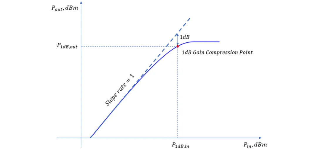 1dB增益压缩点概述及测试
半导体器件是现代电子工业中十分耀眼的明星,近几十年得到了长足的发展,凭借诸多优势,已广泛应用于控制、转换、放大、运算等功能电路,一直以来备受人们的青睐。爱它就要接受它的缺点,任何事物都有自己的缺点,半导体器件也不例外。对于本文所涉及的射频放大器等有源器件,非线性就是其缺点之一。
2020-08-10
下一篇
 Fawkes
给图片穿上“隐身衣”,帮你保护照片隐私数据
2020-08-09